Logistic Regression Simplified

Logistic Regression is one of the most popular machine learning algorithms used for classification problems. Its comes under supervised learning, it helps us predict which category an observation belongs to.

Some common examples include:

• Will a student pass or fail?

• Is an email spam or not spam?

• Will a customer buy a product or not?

• Is a transaction fraudulent or legitimate?

  
  

Instead of directly predicting a category, Logistic Regression first predicts the probability of an event occurring and then converts that probability into a final prediction.

For example, if a model predicts:

Probability of Passing = 92%

the final prediction would be Pass

Throughout this blog, we'll use a simple example to understand how Logistic Regression works.

Meet Jay, a student preparing for his exams. We have information such as:

• Study Hours

• Attendance Percentage

• Mobile Usage

Using these factors, our goal is to predict whether Jay will Pass/Fail

This may sound simple, but it will help us understand every important concept behind Logistic Regression.

Let's start by understanding how Logistic Regression uses information about Jay to make a prediction.

Step 1: Calculating the Score (Weighted Sum - z)

Before Logistic Regression can predict whether Jay will pass or fail, it first needs a way to combine all the information available about him.

Let's look at Jay's details:

Feature	Value
Study Hours	5
Attendance	90%
Mobile Usage	2 Hours

Now think like a teacher.

Would you treat all these factors equally?

Probably not.

You would likely think:

• Study Hours are very important.

• Attendance is important.

• Mobile Usage may have a negative impact if it's too high.

  
  

Logistic Regression thinks in a very similar way.

It assigns an importance value, called a weight, to every feature.

For example:

Feature	Value	Weight
Study Hours	5	+3
Attendance	90	+1
Mobile Usage	2	-2

Notice that Mobile Usage has a negative weight because higher mobile usage may reduce the chances of passing.

You might ask how did it come up with these weights? So initially it assigns random weights and as it learns it keeps on updating them, we will learn about this in detail in the upcoming sections.

Now the model combines everything into a single score called z.

Formula

z = w1​x1​ + w2​x2​ + w3​x3 ​+ b

where:

• x = Feature Value

• w = Weight (importance of the feature)

• b = Bias (starting point of the model)

Using our example:

z = (3    5) + (1   90) + (-2 * 2) + b = 101 + b

Think of z as a confidence score.

A large positive z usually means, Jay is likely to pass.

A large negative z usually means, Jay is likely to fail.

You may have noticed an extra term called b in the formula, this value is called the bias. Think of it as the model's starting point before considering any of Jay's features. Just like weights, the model learns the best value for bias during training. We'll revisit bias later in this blog.

Step 2: Converting the Score into a Probability (Sigmoid Function)

In the previous section, we learned that Logistic Regression combines all the features and creates a score called z.

But there is one problem with a score like:

7

20

100

-10

is difficult to interpret what is the final result, pass/fail?.

What we really want is a probability such as:

95% chance of passing

or

20% chance of passing

This is where the Sigmoid Function comes in.

The Sigmoid Function takes any value of z and converts it into a probability between 0 and 1.

Sigmoid Formula

σ(z) = 1/(1+e^(-z)

Don't worry about the formula for now.

The important thing to remember is what it does.

z Value	Probability
-10	~0%
-1	27%
0	50%
1	73%
7	~99.9%

Notice the pattern:

• Large positive z → Probability close to 1

• Large negative z → Probability close to 0

• z = 0 → Probability = 50%

You may have noticed something interesting.

If z = 0, the Sigmoid Function returns a probability of 50%.

Does that mean a student who doesn't study at all still has a 50% chance of passing?

Not necessarily.

This is where the Bias (b) comes into the picture, it acts like the model's starting point and shifts the value of z up or down before it is passed to the Sigmoid Function.

For example, if the model learns a bias of -5, then even when all feature values are 0:

z= 0+(−5) = −5

The Sigmoid Function would then produce a very low probability (around 1%), which is much more realistic.

In simple terms, bias helps the model make sensible predictions even when all feature values are zero.

Now let's decode the Sigmoid formula

Suppose:

z = 7

The formula becomes:

σ(z) = 1/(1+e^(-7)

Now:

e^(-7) ≈ 0.0009

So:

1/(1+0.0009) ≈ 0.999

or about:

99.9%

This is why a large positive value of z produces a probability very close to 1.

The important thing to remember is that no matter how large or small z becomes, the Sigmoid Function always produces a value between 0 and 1.

Step 3: Making the Final Decision (Threshold)

In the previous step, the Sigmoid Function converted Jay's score into a probability.

While probabilities are useful, we ultimately want a clear answer:

Pass or Fail?

This is where a Threshold comes in.

A threshold is simply a cutoff value used to convert a probability into a final prediction.

The most common threshold is 0.5 (50%)

For Jay, if the model predicts:

Probability = 0.85

Since 0.85 > 0.5

the final prediction becomes pass

Can the threshold be changed?

Absolutely. While 0.5 is the most common threshold, it can be adjusted based on the problem.

• Lower threshold → More positive predictions

• Higher threshold → Fewer positive predictions

For example, in disease detection, we may use a lower threshold to avoid missing patients, while in spam detection, we may use a higher threshold to avoid marking genuine emails as spam.

Step 4: Measuring How Wrong the Prediction Was (Log Loss)

At this point, our model can predict whether Jay will pass or fail.

Let's say the model predicts probability of passing = 90%

But how does the model know whether this prediction was good or bad?

To answer that question, Logistic Regression uses a metric called Log Loss.

Think of Log Loss as a penalty score. The further the prediction is from the actual answer, the larger the penalty.

Let's look at a few examples where the actual result is Jay Passed

Model Prediction	Log Loss
99% Pass	Very Small
80% Pass	Small
60% Pass	Moderate
10% Pass	Very Large

Notice something important:

The model receives the largest penalty when it is confidently wrong.

Log Loss Formula

Log loss = -[y log (p)+(1-y) log(1-p)]

where:

• (y) = Actual Result (0 or 1)

• (p) = Predicted Probability

  
  

Don't worry about memorizing this formula.

The important thing to understand is that:

• Good predictions produce a small loss.

• Bad predictions produce a large loss.

• Confident mistakes produce a very large loss.

The model's goal during training is simple:

Find the set of weights that produces the smallest possible Log Loss.

Now that the model can measure how wrong its predictions are, the next step is to learn from those mistakes and improve the weights.

That's where Gradient, Learning Rate, and Weight Updates come in.

Step 5: Learning from Mistakes (Gradient)

After making a prediction, the model calculates the Log Loss.

Suppose Jay actually passed the exam, but the model predicted:

10% chance of passing

This results in a large loss, which tells the model:

"Something is wrong. We need to adjust the weights."

But there is another question:

• Which weight caused the error?

• Was the weight for Study Hours too small?

• Was the weight for Attendance too large?

• Should Mobile Usage have a stronger negative impact?

This is exactly what the Gradient helps us determine.

Think of the Gradient as a guide that tells the model which direction should I move to reduce the loss?

A simple analogy is climbing down a mountain.

Imagine you're standing on a mountain, and your goal is to reach the bottom. You would naturally look around and move in the direction that takes you downhill fastest.

The Gradient works in a very similar way.

For every weight, the Gradient calculates:

• Whether the weight should increase or decrease.

• How much influence that weight had on the error.

Step 6: How Big Should the Step Be? (Learning Rate)

The Gradient tells the model which direction will reduce the loss.

But there's still one decision left, how big should the next step be?

This is controlled by the Learning Rate.

Think of it as the step size used while learning.

• A very small learning rate makes learning slow.

• A very large learning rate may cause the model to overshoot the optimal solution.

The goal is to find a learning rate that helps the model learn efficiently without taking steps that are too small or too large.

Learning Rate is something that we can set. Suppose it is 1, then in the next learning cycle the weights can be increase/decreased by 1.

At this point we know:

• Log Loss tells us how wrong the prediction is.

• Gradient tells us which direction to move.

• Learning Rate decides how big the step should be.

Now let's see how the model uses all of this information to update its weights.

Step 7: Updating the Weights

The model now has everything it needs. Using this information, the model updates its weights.

Let's say the current weight for Study Hours is:

Weight = 3

Learning rate = 0.1

Gradient = -2

New Weight= Old Weight − (Learning Rate × Gradient)

After calculating the loss and gradient, the model may realize that increasing the importance of Study Hours could improve future predictions.

The updated weight become:

Weight = 3.2

Similarly, the weights for Attendance and Mobile Usage may also be adjusted.

This process is called a Weight Update.

The goal is simple:

Make small improvements to the weights so that the next prediction produces a lower loss.

The model repeats this process again and again, with each update, the model gradually learns which features are important and how much influence they should have on the final prediction

But you might ask how many times does this process repeat?

That's what we'll learn next when we discuss Iterations and Epochs.

Step 8: Repeating the Learning Process (Iterations & Epochs)

As we saw the model does not learn everything in a single step. Instead, it repeats the following process again and again:

Predict -> Calculate Loss -> Update Weight

Each time the model updates its weights, it is called an Iteration.

Now imagine our dataset contains information for 1,000 students.

When the model has seen all 1,000 students once, it completes one Epoch.

In simple terms:

• Iteration = One weight update

• Epoch = One complete pass through the dataset

The model usually needs multiple epochs before it learns the best weights.

With each epoch, the model gradually reduces the loss and improves its predictions.

Step 9: When Does the Model Stop Learning? (Convergence & max_iter)

As the model goes through more and more epochs, the weights gradually improve and the Log Loss gets smaller.

Eventually, the model reaches a point where further weight updates produce very little improvement.

This point is called Convergence.

In simple terms:

The model has learned enough and cannot improve much further.

To prevent the model from training forever, Logistic Regression uses a parameter called max_iter (Maximum Iterations).

It defines the maximum number of learning steps the model is allowed to perform.

For example:

LogisticRegression(max_iter=100)

Here, the model can perform up to 100 iterations while trying to find the best weights.

In most cases, the model reaches convergence before hitting this limit.

If it doesn't, Scikit-Learn may show a warning suggesting that you increase the value of max_iter.

The key takeaway is:

• Convergence = The model has learned enough.

• max_iter = The maximum number of learning steps allowed.

Python Implementation

Now that we understand the theory behind Logistic Regression, let's see how to implement it in Python.

In upcoming blogs, we'll work through real-world use cases and dive deeper into each step of the machine learning workflow. For now, we'll continue with our student exam example to build a basic understanding of how Logistic Regression is implemented in practice.

Step 1: Import Required Libraries

import pandas as pd

from sklearn.model_selection import train_test_split
from sklearn.preprocessing import StandardScaler
from sklearn.linear_model import LogisticRegression

from sklearn.metrics import (
    accuracy_score,
    precision_score,
    recall_score,
    f1_score,
    confusion_matrix
)

Step 2: Load the Dataset

df = pd.read_csv("students.csv")

We are reading a csv file called students, I'll share link to this file towards end of the python implementation section.

Step 3: Define Features (X) and Target (y)

X = df[["StudyHours", "Attendance", "MobileUsage"]]

y = df["Passed"]

Here we are separating features and target so the model can learn patterns using the input features (X) and try to predict target variable (y).

Step 4: Split the Data into Training and Testing Sets

X_train, X_test, y_train, y_test = train_test_split(
    X,
    y,
    test_size=0.2,
    random_state=42
)

Now we split our data into training and testing sets. Training is done on the training set and then we compare it with test set to see how well the model performed.

test_size= 0.2 means 80% is training set and 20% is testing set.

Step 5: Feature Scaling

scaler = StandardScaler()

X_train = scaler.fit_transform(X_train)
X_test = scaler.transform(X_test)

Step 6: Train the Logistic Regression Model

model = LogisticRegression()

model.fit(X_train, y_train)

Step 7: Make Predictions

y_pred = model.predict(X_test)

Step 8: Predict Probabilities

y_prob = model.predict_proba(X_test)

y_prob[:5]

This will return 2 values, 1st probability of passing and 2nd probability of failing.

Step 9: Evaluate the Model

print("Accuracy :", accuracy_score(y_test, y_pred))
print("Precision:", precision_score(y_test, y_pred))
print("Recall   :", recall_score(y_test, y_pred))
print("F1 Score :", f1_score(y_test, y_pred))

Step 10: View Learned Weights and Bias

print("Coefficients:", model.coef_)
print("Bias:", model.intercept_)

Step 11: Predict Whether Jay Will Pass

jay = pd.DataFrame({
    "StudyHours": [5],
    "Attendance": [90],
    "MobileUsage": [2]
})

# Apply the same scaling used during training
jay_scaled = scaler.transform(jay)

# Predict probability
pass_probability = model.predict_proba(jay_scaled)[0][1]

# Predict final class
prediction = model.predict(jay_scaled)[0]

print(f"Pass Probability: {pass_probability:.2%}")
print(f"Prediction: {'Pass' if prediction == 1 else 'Fail'}")

Notebook and Dataset link - AIML/Logistic Regression at main · ishan1510/AIML

Understanding Important LogisticRegression() Parameters

So far, we've trained a Logistic Regression model using:

model = LogisticRegression()

While this works perfectly fine, Logistic Regression provides several parameters that allow us to control how the model learns.

Let's understand the most important ones.

1. penalty — How Should the Model Control Overfitting?

Imagine we train a model and it learns the following weights:

Feature	Weight
Study Hours	25
Attendance	18
Mobile Usage	-22

These weights are quite large. Large weights often indicate that the model is trying too hard to fit the training data, which can lead to overfitting.

Regularization helps prevent this by discouraging excessively large weights. The penalty parameter controls the type of regularization used, lets see them one by one

L2 Regularization (Default)

model = LogisticRegression(
penalty='l2'
)

L2 gently pushes large weights toward zero.

Example:

25  →  8

18  →  5

-22 → -7

The model still uses all features, but with more reasonable weights.

This is the most commonly used option and works well for most problems.

L1 Regularization

model = LogisticRegression(
penalty='l1',
solver='liblinear'
)

L1 is more aggressive.

It can reduce some weights all the way to zero.

Example:

Study Hours  = 12

Attendance   = 0

Mobile Usage = -8

A weight of zero means that feature is effectively ignored by the model.

This makes L1 useful when you have many features and want automatic feature selection.

ElasticNet

model = LogisticRegression(
penalty='elasticnet',
solver='saga'
)

ElasticNet combines the behavior of both L1 and L2 regularization.

It is typically used for larger and more complex datasets.

2. C — How Strict Should Regularization Be?

Now that we understand regularization, the next question is how much regularization should we apply?

This is controlled by the C parameter.

model = LogisticRegression(C=1.0)

Think of C as the amount of freedom given to the model.

If C is Small (C = 0.01)

• Strong regularization

• Smaller weights

• Simpler model

• Lower risk of overfitting

If C is large (C = 100)

• Weak regularization

• Larger weights allowed

• More complex model

• Higher risk of overfitting

3. solver — How Should the Model Find the Best Weights?

During training, Logistic Regression needs an optimization algorithm to find the best weights.

This is controlled by the solver parameter.

model = LogisticRegression(solver='lbfgs')

Think of a solver as the strategy used to find the best weights that minimize Log Loss.

Common Solvers

Solver	When to Use
lbfgs	Default, works for most problems
liblinear	Small datasets, supports L1
saga	Large datasets, supports L1, L2 and ElasticNet

4. max_iter — How Long Should the Model Be Allowed to Learn?

Earlier, we learned about convergence.

The model keeps learning until either:

• It converges, or

• It reaches the maximum number of iterations.

This limit is controlled by max_iter.

model = LogisticRegression(max_iter=1000)

5. class_weight — How Should We Handle Imbalanced Data?

Consider the following dataset:

Result	Count
Pass	990
Fail	10

The model may become biased toward predicting pass, because it sees far more examples of that class.

To handle this, we can use:

model = LogisticRegression(class_weight='balanced')

The model automatically gives more importance to the minority class during training.

Let's see the available class weight options

Default

class_weight=None

All classes are treated equally.

Balanced

class_weight='balanced'

Automatically adjusts class importance based on class frequencies.

Most commonly used for imbalanced datasets.

Custom Weights

class_weight={

    0: 1,

    1: 5

}

Useful when one class is significantly more important than the other.

Examples:

• Fraud Detection

• Disease Detection

• Defect Detection

where missing a positive case can be costly.

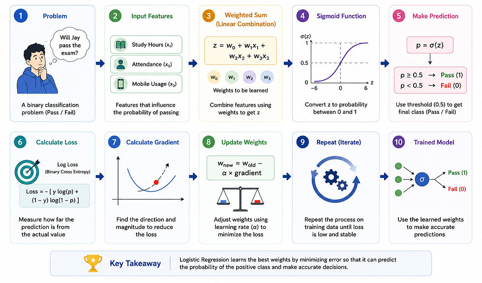
Summarizing What We Learnt

Conclusion

Congratulations! 🎉

You now understand how Logistic Regression works from both a mathematical and practical perspective.

We started with a simple question — Will Jay pass the exam? — and used it to explore concepts such as weighted sums, sigmoid, thresholds, log loss, gradients, learning rate, weight updates, model training & Python implementation.

The most important thing to remember is that Logistic Regression is not just a formula—it is a learning process. The model continuously makes predictions, measures its mistakes, and adjusts itself until it finds the best possible weights.

While Logistic Regression is one of the simplest machine learning algorithms, it forms the foundation for understanding many advanced machine learning and deep learning techniques.

In the next blogs, we'll apply these concepts to real-world datasets and explore more models in detail.

See you in the next blog — stay curious, keep growing. 🚀